
Measures of centrality:
MEAN, MEDIAN, & MODE
Module learning objectives
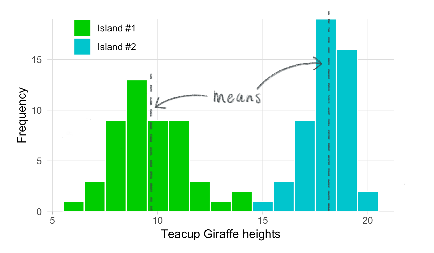
You’ve just collected a lot data and graphed heights. Although informative, a graphical display of these data is difficult to summarize – we need to describe these heights with a single number that will be meaningful and allow us to do statistics.
We can do this with a measure of centrality, the concept that one number in the “center” of the data set is a good summary of all the values. Below are examples of different measures of centrality.
The mean is the average and the measure of centrality that you are probably most familiar with. This is a good measure to use when the data are normally distributed. We describe it in detail below.
The median is the value in the middle of the data set. Half of the observations lie above the median and half below. When the data are normally distributed, the median and the mean will be very close to each other. When your data are not normally distributed (skewed to the left or right) the median is a more appropriate measure of centrality (see the animation below).
The mean of a variable is the sum of its values, divided by the number of values.
This concept can be represented with equation below. In our case, each “x” represents a giraffe height (i.e. a single observation), and the numerical subscript indicates its order in the sample. We’ll use \({\bar{x}}\) (read “x-bar”) to represent the mean of the height variable.
To make this more efficient, instead of writing “\({x_1 + x_2 + ... + x_n}\)”, we can use the uppercase sigma symbol \(\sum{}\) to represent summation of all the observations.
\[\begin{equation} \tag{2} \Large{\bar{x}} = \frac{\sum_{i=1}^{n}{x_i}}{n} \end{equation}\]
This might look intimidating, but equation (2) is really showing the same thing as (1). Let’s go through the steps again, breaking the symbols apart a bit (see annotated equation (3) below). The sigma means ‘add up’. What are we adding up? All the heights “x”. The “i = ” part indicates which term to begin with. For our purposes, this will always be the first observation, hence \(i\) = 1. The character on top of the sigma is the last observation we include in our summation. In this case it’s n – because we’re adding all n = 50 observations in each group of giraffes. In both equations, we still divide by the total number of observations in each group we have: again, n.
Recall our discussion about a sample versus a population. Different symbols are used to represent the mean for each of these. We’ve already discussed \(\bar{x}\) for the sample mean. The analogous symbol for the population mean is \({\mu}\) (read “mu”). Additionally, when referring to the size of the population, we will use a capital \({N}\) instead of a lowercase one.
heights_island1. Below we show the first few observations from this vector, using the head() function.
head(heights_island1)## [1] 7.038865 13.154339 8.086511 8.159990 6.004716 9.455408
Use the interactive window below to calculate the mean “by hand”.
Now it’s your turn to write your own function. Call it “my_mean” and have it calculate the mean of any given vector. You’re going to use the rules for writing a function in R that you’ve used previously. As a reminder, you’ll use function() and embed your code (that you completed in the window above) within curly brackets{}. The advantage of making a “homemade” function is that you can string together all the steps from the previous exercise into a single command.
You can also complete the exercise above in RStudio on your local computer. This way you will be able to save your my_mean() function and script for future use.

To calculate the median go through the following steps:
Before you write your own median function, two concepts need to be introduced: 1) the modulus operator %% and 2) if...else statements.
11 %% 5 returns the 1, which is the remainer of 11 divided by 5. If the modulus operation returns 0, then there is no remainder. It is useful to apply the modulus operation x %% 2 to determine whether a number x is even or odd by testing if the result is exactly equal to 0. See example code below.
> 10 %% 2## [1] 0> 10 %% 2 == 0## [1] TRUE> 11 %% 2## [1] 1> 11 %% 2 == 0## [1] FALSE
An if...else statement is useful when you want to specify distinct outcomes for objects dependent on whether they meet your set criteria. See below.
Now that you have a sense for how the %% operator can be used to test whether a number is EVEN or ODD, and how if...else statements work, use both of these concepts in the window below to write your own function that calculates the median of any vector.
Remember that the sample mean is an estimate of the entire population’s mean (which would often be impossibly large to measure). How reliably does the mean of a sample represent the population mean? Warning: if a small sample has been used, the sample mean may not be a reliable at all! Estimates from small samples are subject to the whims of randomness. On the other hand, the larger the sample, the closer the sample size appraches the population size, and the more reliable the sample estimate becomes.
Pressing ‘Play’ on the plot below will illustrate this concept.
For further reading see the Law of Large Numbers.
This project was created entirely in RStudio using R Markdown and published on GitHub pages.