
Introduction to Inference:
Standard Error
Module learning objectives
Let’s revisit the first few days during which we collected data stored in the vector heights_island1. We were able to verify that the heights were normally distributed and calculated our sample mean, \({\bar{x}}\). However, we know that \({\bar{x}}\) is only an estimate of the true population mean, \({\mu}\), which is the true value of interest. It is unlikely that we will ever know the value of \({\mu}\), since access to all possible observations is rare. Therefore we will have to rely on \({\bar{x}}\) estimates from random samples drawn from the population as the best approximation of \({\mu}\).
Not all sample means are created equal. Some are better estimates than others. Recall the animation showing the relationship between sample size and variability of the mean. As we learned from this animation, in the long-run, large samples are necessary to get an accurate estimate of \({\mu}\).
A note about language: here, words like “accuracy”, “precision”, and “uncertainty” are used in a rather fast and loose way. We’re using the laymen’s application of these terms to refer to the long-run variability of estimates produced from repeated, independent trials. There are stricter, more formal statistical uses for these words, but for right now, we’re going to ignore these nuances so that we can move on with understanding these concepts in broad strokes.
One reason we care about our sample estimate’s accuracy is because we want to be able to answer questions about the population by making inferences. Statistical inference uses math to draw conclusions about the population based on a subset of the full picture (i.e. a sample). Subsets of data are of course limited, so it’s therefore important to acknowledge that the strength of the conclusions drawn about the population is dependent on the precision of the sample estimate. For example, say that we guess that the population mean value of giraffe heights on Island 1 is less than 11 cm. We can make some inferences about whether or not this is a good guess based on what we learn from our sample of giraffe heights. We’ll revisit this question a few times below.
The mean of our sample of 50 giraffes from Island 1 was:
mean(heights_island1)## [1] 9.714141How can we quantify the accuracy of this estimate, given its sample size?
In theory, one way to illustrate this is to generate data not just from a single sample but from many samples of the same size (N) drawn from the same population.
Imagine that after you collected all 50 measurements for heights_island1, you wake up one morning with no memory of collecting data at all—and so you go out and collect 50 giraffe heights again and subsequently calculate the mean. Further imagine that this groundhog day (or more correctly, groundhog week) situation repeats itself many, many times.
When you finally return to your sanity, you find stacks of notebooks filled with mean values from each of your individual data collections.

Instead of viewing this as a massive waste of time, you make the best out of the situation and create a histogram of all the means. In other words you create a plot showing the distribution of the sample means, also known as a sampling distribution.
The animation below illustrates the process of creating the sampling distribution for 1,000 sample means.
On the left side, each histogram represents a sample (e.g. heights_island1 would be one sample, and we’re flashing through 1,000 of them in total). Correspondingly, each dot signifies an observation. After each sample histogram is completed, \({\bar{x}}\) is calculated. This \({\bar{x}}\) value is then subsequently added to the histogram of the sampling distribution on the right. As you can see below, this process is repeated, allowing the sampling distribution to build up.
A histogram of the sampling distribution is shown below. It is a histogram made up of many means.
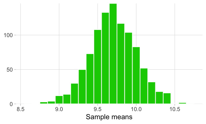
Looking at the spread of \({\bar{x}}\) values that this groundhog experience generated, we can get a sense of the range of many possible estimates of \({\mu}\) that a sample of 50 giraffes can produce.
The sampling distribution provides us with the first hint of the precision of our original heights_island1 estimate, which we’ll quantify in more detail later on, but for now it’s enough to notice that the range of possible \({\bar{x}}\) values are between 8.9 and 10.7. This means that \({\bar{x}}\) values outside of this range are essentially improbable.
Let’s return to our question about whether the true mean of giraffe heights on Island 1 is less than 11 cm. Our sampling distribution suggests that \({\mu}\) is less than 11 cm, since values greater than that are not within the range of this sampling distribution.
Back to the idea that larger samples are “better”, we can explore what happens if we redo the groundhog scenario, this time sampling 500 individuals (instead of 50) before taking the mean each time, repeating this until thousands of \({\bar{x}}\) values have been recorded. For completeness, let’s imagine the same marathon data collection using samples that are smaller—of 5 giraffes each. We compare the resulting sampling distributions from all three scenarios below. The middle sampling distribution corresponds to the sampling distribution we already generated above.
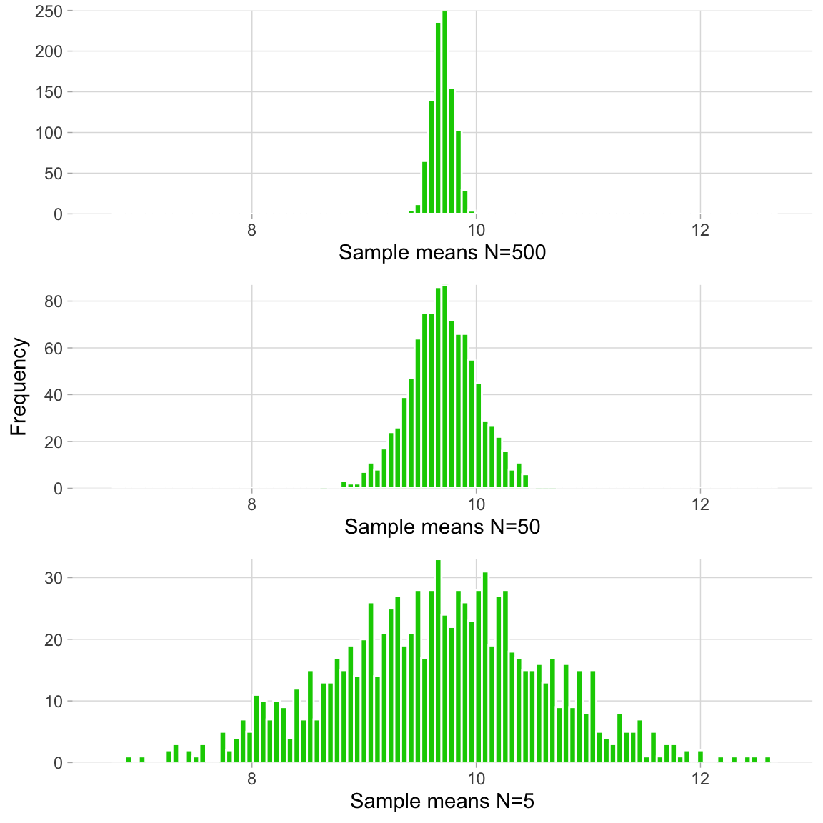
What do we notice?
We can take the mean of the sampling distribution itself– the mean of the sampling distribution is a mean of means. This mean can be interpreted to be the same as a mean that would have resulted from a single large sample, made up of all the individual observations from each of the samples whose \({\bar{x}}\) values are included in the sampling distribution.
Note that if we had only generated a sampling distribution made up of samples of 5 giraffes, we would not have been able to exclude 11 cm as a possible value for \({\mu}\). In fact, if we were to draw a vertical line in the middle of each of the sampling distributions (the mean), we can tell that the population mean is likely even less than 10 cm.
In the following window, you will test the relationship between sampling distribution and sample size. The function below (behind-the-scenes code not shown) will plot a sampling distribution made up of 1000 samples, with each sample containing N number of observations. Try setting N to a few different values. What does the resulting sampling distribution looks like? See if you can confirm for yourself that the above points are true.
As we’ve done before, we want to summarize this spread of mean estimates with a single value. We’ve already learned how to quantify a measure of spread–the standard deviation. If we take the standard deviations of each of the three different sampling scenarios above, then we accept that distributions based on smaller samples should have larger standard deviations.
In the window below, calculate the standard deviation of each of the three sampling distributions (i.e. for N = 500, N = 50, and N = 5), and confirm that the italicized point above is true. (If you’re working in R locally, use your “homemade” standard deviation function from the Variance module.)
To complete this exercise, you will need to use the objects sampling_distribution_N500, sampling_distribution_N50, sampling_distribution_N5, which are vectors storing the thousands of \({\bar{x}}\) values from the corresponding groundhog sampling distributions.
When you calculate the standard deviation of a sampling distribution of \({\bar{x}}\) values, you are calculating the standard error of the mean (SEM), or just “standard error”. The SEM is the value that we use to capture the level of precision of our sample estimate. But, we need a better and more efficient way to arrive at this value without relying on a groundhog day situation. Keep reading to learn more.
A note about SEM: Here “standard error” will imply standard error of the mean. But we can technically calculate the standard error of any sample statistic, not just the mean. We’ll talk about that more in future modules.

Deriving the equation used for calculating the standard error of the mean using theory (i.e. without going out and resampling MANY times) is a bit complicated, but if you’re interested, you can learn more about it here. Instead, we can capture the relationship between standard deviation, sample size, and standard error with the plot below.
The standard deviation in this plot is 2.1, which represents \({\sigma}\) for giraffe heights on Island 1. This population value is technically still unknown but can be deduced in theory by repeating the groundhog day example for the standard deviation instead of for the mean. It’s important to note that the plot would have the same shape regardless of what scenario or standard deviation we were using.
Can you figure out what the equation is for the SEM? Look at the plot above, hover over the points, and see if you can gather how standard error of the mean, standard deviation, and sample size are related. Here are some hints:
Use the window below as a calculator to see if you can figure out the equation for the SEM.
In case you weren’t able to figure it out, remember to check the Solutions tab in the exercise window or take a look at this link for the equation for calculating the SEM. Recall that we’re working with the sample (and not population) standard deviation (\(s\)), so make sure you find the correct equation.
Let’s test out the SEM equation on our original sample of heights_island1 and compare it to what we would have gotten by taking the standard deviation of the sampling distribution example with the N= 50 case. Does the SEM seem like a good approximation of the standard deviation of the sampling distribution?
Below, you will use the object heights_island1, which contains our single sample of N=50, and the object sampling_distribution_N50, which contains the data from the corresponding groundhog sampling distribution.
Close enough! We wouldn’t expect these to be exactly the same because of sampling variability.
Now that we have a better understanding of how to gauge the precision of our sample estimates, we can test our question about the \({\mu}\) being less than 11 cm once and for all.
To formally make inferences, we need to revisit the principles of the empirical rule to construct confidence intervals. (Confidence intervals are just one way to make inferences– we’ll discuss other ways later.)
Remember, that the SEM is just the standard deviation of the sampling distribution, so we can apply the empirical rule. As a result, ± 2 SEM from a point estimate will capture ~95% of the sampling distribution. Actually, we were a little bit sloppy earlier when we said 2 standard deviations captures 95% of a normal distribution; this will actually give you 95.45% of the data. The true value is 1.96 standard deviations–and this is what we use to construct a 95% confidence interval (CI).
Loosely speaking, a 95% CI is the range of values that we are 95% confident contains the true mean of the population. We want to know whether our guess of 11 cm falls outside of this range of certainty. If it does – we can be sure enough that the true \({\mu}\) of giraffe heights on Island 1 is less than 11 cm.
Use the window below to find out and make your first inference by constructing the 95% CI for the heights_island1 mean estimate!
The upper limit of our 95% CI is less than 11 cm, so the population mean of heights on island 1 is likely less than 11 cm. In the scientific community, this is a bonafide way of drawing this conclusion.

We’ve been a little fast and loose with our words. The formal definition of CIs is the following:
If we were to sample over and over again, then 95% of the time the CIs would contain the true mean.
Importantly, some examples of what the 95% CI does NOT mean are:
The precise interpretation of CIs is quite a nuanced and rather hotly debated topic see here and becomes somewhat philosophical– so if these definition subtleties seem confusing, don’t feel bad. As mentioned in the blog post linked above, one recent paper reported that 97% of surveyed researchers endorsed at least one misconception (out of 6) about CIs.
This project was created entirely in RStudio using R Markdown and published on GitHub pages.